Index-Match!

One of the most common requirements of any desk job is  proficiency at excel and one of the most common excel-related questions is "Do you know Vlookup?". Wouldn't it be great if you can answer something like, "I use Index-Match which I find to be superior to vlookup.". This would immediately tell your interviewer / manager that you are proficient at excel.

Vlookup is great. However, it has a big limitation. You need to specify col_index_num in your formulas and this requires you to count the columns and specify a column number (starting with 1 for the left most column in the array). The column number is a constant. It is not relative in the sense that changes to the number of columns in array table structure might impact the output. More specifically, when a column is deleted or added to the left of the column specified in the vlookup formula, the output changes accordingly.

Index-Match overcomes this problem by providing a relative reference to the column in question.

Here is an example:

Look Up 1 and Output Column is an array A1:B6 with 2 columns and 5 rows (excluding headers).
Look Up 2 and Need Output here are the columns where we need to look up c and e to extract the values from A1:B6 i.e. 2,000 and 3,000.

The formula in F2 would be

=INDEX(Output Column,MATCH(Look Up 2 item ,Look Up 1 column, match exactly))

or

=INDEX($B$2:$B$6,MATCH($E2,$A$2:$A$6,0))

I remember this formulas as index - select the column from which you need the output, now match your look up item in the column with look up items and match exactly i.e. with zero differences.

Drag the formula to column F3 (or copy-paste) and you retrieve the value 3,000.

If you are already familiar with either Index or Match functions, the below isn't for you. 

Now let's learn a little more about Index & Match functions.

Index Function:

Index function goes to a specified row & column (optional), in that order, in the array and gives you the output. 

= INDEX(array, row_num, [column_num])

In the above example, if we know the row number, we can input the below formula in cell F2:

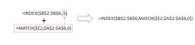
 =INDEX($B$2:$B$6, 3) or =INDEX($B$2:$B$6, 3,1)

However, we might as well directly link the output cell if we know the row number. This would be a big pain if your output column has hundreds of rows. You want excel to search for the right row and give you the output. 

Match Function:

This is where the Match function comes in handy. It does the search for you.

=MATCH(lookup_value, lookup_array, [match_type])

In this case, we know the look_value i.e. C. We know the lookup_array i.e. Look Up 1 column.The match type 0 looks for an exact match.

Continuing with the example, our match formula is:

=MATCH($E2,$A$2:$A$6,0) i.e. 3

Now all we need to do is to combine the index and match formulas. The 3 in the INDEX formula is replaced by the MATCH formula.

You can use the index match formula for hlookups. In this case your match function will look up the column number.

Your feedback is much appreciated and be sure to brag about your 'look up' skills. We will talk about the $ signs in the formulas in the following post.

Excel at Excel!

This excel blog is dedicated to an everyday finance professional and college students.

In the recent year, I've interviewed candidates fresh off the college as well as candidates with 1 to 3 years of finance analyst / accountant experience.

Proficiency in excel is one of the basic job requirements. And, I was surprised at how many of these candidates were lacking basic skills. I could tell that they have learnt excel in their college or had some experience but the experience that you get working in real scenarios is different.

Here are some of the advantages of being great with excel (based on my experience):

• Ace the interviews: If there is one thing about your interview that you knock out of the park, it is excel. You would want to have an intelligent conversation about excel right from the beginning. This makes the interviewer comfortable about your skills and he / she would quickly move on to the other areas. Any signs of incompetence in this area will most likely weaken the candidates chances of getting hired.
• Get your work done faster
• Impress your manager / peers: Often, your manager / peers will sit with you while working / reviewing a financial model. Would you like to impress them with your knowledge? If yes, this blog is for you. I owe my success in the beginning stages of my career to this. I was the go to person for complex financial models, automated templates and anything that involves getting things done quickly on excel. You peers might not say it out but they sure think you are a super star at excel. 
• More responsibility: Getting your work done faster on excel and impressing your team with your excel skills will mean that you will be a valuable resource and more and more work will come to you. In your early stages at work, this is very valuable as you often get insights in to areas of business that you would otherwise not get exposed to.

We are both professionals who use Excel on a daily basis, and hit new problems every day. We hope to share our learning by demonstrating actual situations we faced at work, and how we used Excel to solve it.

If you would like to recommend / learn different topics, please reach out to us. You feedback is valuable and is highly appreciated.